Tutorials

Getting Started with DMRG

The density matrix renormalization group (DMRG) is an algorithm for computing eigenstates of Hamiltonians (or extremal eigenvectors of large, Hermitian matrices). It computes these eigenstates in the matrix product state (MPS) format.

Let's see how to set up and run a DMRG calculation using the ITensor library. We will be interested in finding the ground state of the quantum Hamiltonian $H$ given by:

\[H = \sum_{j=1}^{N-1} \mathbf{S}_{j} \cdot \mathbf{S}_{j+1} = \sum_{j=1}^{N-1} S^z_{j} S^z_{j+1} + \frac{1}{2} S^+_{j} S^-_{j+1} + \frac{1}{2} S^-_{j} S^+_{j+1}\]

This Hamiltonian is known as the one-dimensional Heisenberg model and we will take the spins to be $S=1$ spins (spin-one spins). We will consider the case of $N=100$ and plan to do five sweeps of DMRG (five passes over the system).

ITensor DMRG Code

Let's look at an entire, working ITensor code that will do this calculation then discuss the main steps. If you need help running the code below, see the getting started page on Running ITensor and Julia Codes.

using ITensors
let
  N = 100
  sites = siteinds("S=1",N)

  ampo = OpSum()
  for j=1:N-1
    ampo += "Sz",j,"Sz",j+1
    ampo += 1/2,"S+",j,"S-",j+1
    ampo += 1/2,"S-",j,"S+",j+1
  end
  H = MPO(ampo,sites)

  psi0 = randomMPS(sites,10)

  sweeps = Sweeps(5)
  setmaxdim!(sweeps, 10,20,100,100,200)
  setcutoff!(sweeps, 1E-10)

  energy, psi = dmrg(H,psi0, sweeps)

  return
end

Steps of The Code

The first two lines

N = 100
sites = siteinds("S=1",N)

tells the function siteinds to make an array of ITensor Index objects which have the properties of $S=1$ spins. This means their dimension will be 3 and they will carry the "S=1" tag, which will enable the next part of the code to know how to make appropriate operators for them.

Try printing out some of these indices to verify their properties:

@show sites[1]

(dim=3|id=704|"S=1,Site,n=1")

The next part of the code builds the Hamiltonian:

ampo = OpSum()
for j=1:N-1
  ampo += "Sz",j,"Sz",j+1
  ampo += 1/2,"S+",j,"S-",j+1
  ampo += 1/2,"S-",j,"S+",j+1
end
H = MPO(ampo,sites)

An OpSum is an object which accumulates Hamiltonian terms such as "Sz",1,"Sz",2 so that they can be summed afterward into a matrix product operator (MPO) tensor network. The line of code H = MPO(ampo,sites) constructs the Hamiltonian in the MPO format, with physical indices given by the array sites.

The line

psi0 = randomMPS(sites,10)

constructs an MPS psi0 which has the physical indices sites and a bond dimension of 10. It is made by a random quantum circuit that is reshaped into an MPS, so that it will have as generic and unbiased properties as an MPS of that size can have. This choice can help prevent the DMRG calculation from getting stuck in a local minimum.

The lines

sweeps = Sweeps(5)
setmaxdim!(sweeps, 10,20,100,100,200)
setcutoff!(sweeps, 1E-10)

construct a Sweeps objects which is initialized to define 5 sweeps of DMRG. The call to setmaxdim! sets the maximum dimension allowed for each sweep and the call to setcutoff! sets the truncation error goal of each sweep (if fewer values are specified than sweeps, the last value is used for all remaining sweeps).

Finally the call

energy, psi = dmrg(H,psi0,sweeps)

runs the DMRG algorithm included in ITensor, using psi0 as an initial guess for the ground state wavefunction. The optimized MPS psi and its eigenvalue energy are returned.

After the dmrg function returns, you can take the returned MPS psi and do further calculations with it, such as measuring local operators or computing entanglement entropy.

Conserving Quantum Numbers (QNs) in DMRG

An important technique in DMRG calculations of quantum Hamiltonians is the conservation of quantum numbers. Examples of these are the total number of particles of a model of fermions, or the total of all $S^z$ components of a system of spins. Not only can conserving quantum numbers make DMRG calculations run more quickly and use less memory, but it can be important for simulating physical systems with conservation laws and for obtaining ground states in different symmetry sectors. Note that ITensor currently only supports Abelian quantum numbers.

Necessary Changes

Setting up a quantum-number conserving DMRG calculation in ITensor requires only very small changes to a DMRG code. The main changes are:

using tensor indices (Index objects) which carry quantum number (QN) information to build your Hamiltonian and initial state
initializing your MPS to have well-defined total quantum numbers

Importantly, the total QN of your state throughout the calculation will remain the same as the initial state passed to DMRG. The total QN of your state is not set separately, but determined implicitly from the initial QN of the state when it is first constructed.

Of course, your Hamiltonian should conserve all of the QN's that you would like to use. If it doesn't, you will get an error when you try to construct it out of the QN-enabled tensor indices.

Making the Changes

Let's see how to make these two changes to the DMRG code from the Getting Started with DMRG tutorial above. At the end, we will put together these changes for a complete, working code.

Change 1: QN Site Indices

To make change (1), we will change the line

sites = siteinds("S=1",N)

by setting the conserve_qns keyword argument to true:

sites = siteinds("S=1",N; conserve_qns=true)

Setting conserve_qns=true tells the siteinds function to conserve every possible quantum number associated to the site type (which is "S=1" in this example). For $S=1$ spins, this will turn on total-$S^z$ conservation. (For other site types that conserve multiple QNs, there are specific keyword arguments available to track just a subset of conservable QNs.) We can check this by printing out some of the site indices, and seeing that the subspaces of each Index are labeled by QN values:

@show sites[1]
@show sites[2]

Sample output:

 sites[1] = (dim=3|id=794|"S=1,Site,n=1") <Out>
 1: QN("Sz",2) => 1
 2: QN("Sz",0) => 1
 3: QN("Sz",-2) => 1
 sites[2] = (dim=3|id=806|"S=1,Site,n=2") <Out>
 1: QN("Sz",2) => 1
 2: QN("Sz",0) => 1
 3: QN("Sz",-2) => 1

In the sample output above, note than in addition to the dimension of these indices being 3, each of the three settings of the Index have a unique QN associated to them. The number after the QN on each line is the dimension of that subspace, which is 1 for each subspace of the Index objects above. Note also that "Sz" quantum numbers in ITensor are measured in units of $1/2$, so QN("Sz",2) corresponds to $S^z=1$ in conventional physics units.

Change 2: Initial State

To make change (2), instead of constructing the initial MPS psi0 to be an arbitrary, random MPS, we will make it a specific state with a well-defined total $S^z$. So we will replace the line

psi0 = randomMPS(sites,10)

by the lines

state = [isodd(n) ? "Up" : "Dn" for n=1:N]
psi0 = productMPS(sites,state)

The first line of the new code above makes an array of strings which alternate between "Up" and "Dn" on odd and even numbered sites. These names "Up" and "Dn" are special values associated to the "S=1" site type which indicate up and down spin values. The second line takes the array of site Index objects sites and the array of strings state and returns an MPS which is a product state (classical, unentangled state) with each site's state given by the strings in the state array. In this example, psi0 will be a Neel state with alternating up and down spins, so it will have a total $S^z$ of zero. We could check this by computing the quantum-number flux of psi0

@show flux(psi0)
# Output: flux(psi0) = QN("Sz",0)

Setting Other Total QN Values

The above example shows the case of setting a total "Sz" quantum number of zero, since the initial state alternates between "Up" and "Dn" on every site with an even number of sites.

To obtain other total QN values, just set the initial state to be one which has the total QN you want. To be concrete let's take the example of a system with N=10 sites of $S=1$ spins.

For example if you want a total "Sz" of +20 (= QN("Sz",20)) in ITensor units, or $S^z=10$ in physical units, for a system with 10 sites, use the initial state:

state = ["Up" for n=1:N]
psi0 = productMPS(sites,state)

Or to initialize this 10-site system to have a total "Sz" of +16 in ITensor units ($S^z=8$ in physical units):

state = ["Dn","Up","Up","Up","Up","Up","Up","Up","Up","Up"]
psi0 = productMPS(sites,state)

would work (as would any state with one "Dn" and nine "Up"'s in any order). Or you could initialize to a total "Sz" of +18 in ITensor units ($S^z=9$ in physical units) as

state = ["Z0","Up","Up","Up","Up","Up","Up","Up","Up","Up"]
psi0 = productMPS(sites,state)

where "Z0" refers to the $S^z=0$ state of a spin-one spin.

Finally, the same kind of logic as above applies to other physical site types, whether "S=1/2", "Electron", etc.

Putting it All Together

Let's take the DMRG code from the Getting Started with DMRG tutorial above and make the changes above to it, to turn it into a code which conserves the total $S^z$ quantum number throughout the DMRG calculation. The resulting code is:

using ITensors
let
  N = 100
  sites = siteinds("S=1",N;conserve_qns=true)

  ampo = OpSum()
  for j=1:N-1
    ampo += "Sz",j,"Sz",j+1
    ampo += 1/2,"S+",j,"S-",j+1
    ampo += 1/2,"S-",j,"S+",j+1
  end
  H = MPO(ampo,sites)

  state = [isodd(n) ? "Up" : "Dn" for n=1:N]
  psi0 = productMPS(sites,state)
  @show flux(psi0)

  sweeps = Sweeps(5)
  setmaxdim!(sweeps, 10,20,100,100,200)
  setcutoff!(sweeps, 1E-10)

  energy, psi = dmrg(H,psi0, sweeps)

  return
end

Getting Started with MPS Time Evolution

An important application of matrix product state (MPS) tensor networks in physics is computing the time evolution of a quantum state under the dynamics of a Hamiltonian $H$. An accurate, efficient, and simple way to time evolve a matrix product state (MPS) is by using a Trotter decomposition of the time evolution operator $U(t) = e^{-i H t}$.

The technique we will use is "time evolving block decimation" (TEBD). More simply it is just the idea of decomposing the time-evolution operator into a circuit of quantum 'gates' (two-site unitaries) using the Trotter-Suzuki approximation and applying these gates in a controlled way to an MPS.

Let's see how to set up and run a TEBD calculation using ITensor.

The Hamiltonian $H$ we will use is the one-dimensional Heisenberg model which is given by:

\[\begin{aligned} H & = \sum_{j=1}^{N-1} \mathbf{S}_{j} \cdot \mathbf{S}_{j+1} \\ & = \sum_{j=1}^{N-1} S^z_{j} S^z_{j+1} + \frac{1}{2} S^+_{j} S^-_{j+1} + \frac{1}{2} S^-_{j} S^+_{j+1} \end{aligned} \]

The TEBD Method

When the Hamiltonian, like the one above, is a sum of local terms,

\[H = \sum_j h_{j,j+1}\]

where $h_{j,j+1}$ acts on sites j and j+1, then a Trotter decomposition that is particularly well suited for use with MPS techniques is

\[e^{-i \tau H} \approx e^{-i h_{1,2} \tau/2} e^{-i h_{2,3} \tau/2} \cdots e^{-i h_{N-1,N} \tau/2} e^{-i h_{N-1,N} \tau/2} e^{-i h_{N-2,N-1} \tau/2} \cdots e^{-i h_{1,2} \tau/2} + O(\tau^3)\]

Note the factors of two in each exponential. Each factored exponential is known as a Trotter "gate".

We can visualize the resulting circuit that will be applied to the MPS as follows:

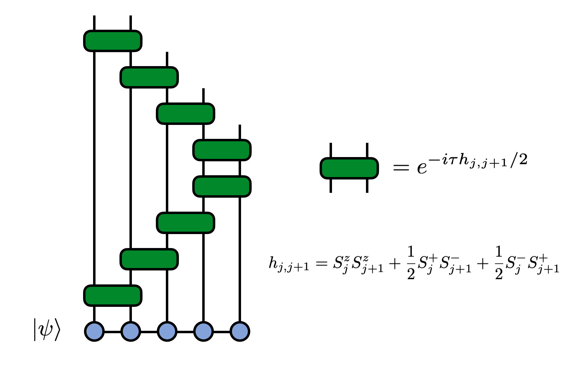
The error in the above decomposition is of order $\tau^3$, so that will be the error accumulated per time step. Because of the time-step error, one takes $\tau$ to be small and then applies the above set of operators to an MPS as a single sweep, then does a number $(t/\tau)$ of sweeps to evolve for a total time $t$. The total error will therefore scale as $\tau^2$ with this scheme, though other sources of error may dominate for long times, or very small $\tau$, such as truncation errors.

Let's take a look at the code to apply these Trotter gates to an MPS to time evolve it. Then we will break down the steps of the code in more detail.

ITensor TEBD Time Evolution Code

Let's look at an entire, working ITensor code that will do this calculation then discuss the main steps. (If you need help running the code below, see the getting started page on running ITensor codes.)

using ITensors

let
  N = 100
  cutoff = 1E-8
  tau = 0.1
  ttotal = 5.0

  # Compute the number of steps to do
  Nsteps = Int(ttotal/tau)

  # Make an array of 'site' indices
  s = siteinds("S=1/2",N;conserve_qns=true)

  # Make gates (1,2),(2,3),(3,4),...
  gates = ITensor[]
  for j=1:N-1
    s1 = s[j]
    s2 = s[j+1]
    hj =       op("Sz",s1) * op("Sz",s2) +
         1/2 * op("S+",s1) * op("S-",s2) +
         1/2 * op("S-",s1) * op("S+",s2)
    Gj = exp(-1.0im * tau/2 * hj)
    push!(gates,Gj)
  end
  # Include gates in reverse order too
  # (N,N-1),(N-1,N-2),...
  append!(gates,reverse(gates))

  # Function that measures <Sz> on site n
  function measure_Sz(psi,n)
    psi = orthogonalize(psi,n)
    sn = siteind(psi,n)
    Sz = scalar(dag(prime(psi[n],"Site"))*op("Sz",sn)*psi[n])
    return real(Sz)
  end

  # Initialize psi to be a product state (alternating up and down)
  psi = productMPS(s, n -> isodd(n) ? "Up" : "Dn")

  c = div(N,2)

  # Compute and print initial <Sz> value
  t = 0.0
  Sz = measure_Sz(psi,c)
  println("$t $Sz")

  # Do the time evolution by applying the gates
  # for Nsteps steps
  for step=1:Nsteps
    psi = apply(gates, psi; cutoff=cutoff)
    t += tau
    Sz = measure_Sz(psi,c)
    println("$t $Sz")
  end

  return
end

Steps of The Code

After setting some parameters, like the system size N and time step $\tau$ to use, we compute the number of time evolution steps Nsteps that will be needed.

The line s = siteinds("S=1/2",N;conserve_qns=true) defines an array of spin 1/2 tensor indices (Index objects) which will be the site or physical indices of the MPS.

Next we make an empty array gates = ITensor[] that will hold ITensors that will be our Trotter gates. Inside the for n=1:N-1 loop that follows the lines

hj =      op("Sz",s1) * op("Sz",s2) +
    1/2 * op("S+",s1) * op("S-",s2) +
    1/2 * op("S-",s1) * op("S+",s2)

call the op function which reads the "S=1/2" tag on our site indices (sites j and j+1) and which then knows that we want the spin 1/ 2 version of the "Sz", "S+", and "S-" operators. The op function returns these operators as ITensors and we tensor product and add them together to compute the operator $h_{j,j+1}$ defined as

\[h_{j,j+1} = S^z_j S^z_{j+1} + \frac{1}{2} S^+_j S^-_{j+1} + \frac{1}{2} S^-_j S^+_{j+1} \]

which we call hj in the code.

To make the corresponding Trotter gate Gj we exponentiate hj times a factor $-i \tau/2$ and then append or push this onto the end of the gate array gates.

Gj = exp(-1.0im * tau/2 * hj)
push!(gates,Gj)

Having made the gates for bonds (1,2),(2,3),(3,4), etc. we still need to append the gates in reverse order to complete the correct Trotter formula. Here we can conveniently do that by just calling the Julia append! function and supply a reversed version of the array of gates we have made so far. This can be done in a single line of code append!(gates,reverse(gates)).

So that the code produces interesting output, we define a function called measure_Sz that we will pass our MPS into and which will return the expected value of $S^z$ on a given site, which we will take to be near the center of the MPS. The details of this function are outside the scope of this tutorial, but are explained in the example code for measuring MPS.

The line of code psi = productMPS(s, n -> isodd(n) ? "Up" : "Dn") initializes our MPS psi as a product state of alternating up and down spins. We call measure_Sz before starting the time evolution.

Finally, to carry out the time evolution we loop over the step number for step=1:Nsteps and during each step call the function

psi = apply(gates, psi; cutoff=cutoff)

which applies the array of ITensors called gates to our current MPS psi, truncating the MPS at each step using the truncation error threshold supplied as the variable cutoff.

The apply function is smart enough to determine which site indices each gate has, and then figure out where to apply it to our MPS. It automatically handles truncating the MPS and can even handle non-nearest-neighbor gates, though that feature is not used in this example.